Writing a Relativistic Raytracer

This is the story of writing a relativistic raytracer (for the third time).

I initially got started on this project back in April of 2022. I love the movie Interstellar, and after watching a video where Scott Manley made a video on traveling through a wormhole. I suddenly became enamored with the idea of rendering a black hole on my own, and set out in search of the tool he used.

Background: Black Holes #

Black holes are incredibly dense objects in space that are so massive they warp spacetime around them. Technically, all matter does this - it’s the reason orbits happen. However, with black holes, they warp space so much that light cannot escape. This is what makes them “black.” They look like dark holes in space, sucking in all matter around them, with no possible escape. Light bends around them, creating the famous warping patterns we see in media.

I wanted to see what they looked like for myself. Since I can’t go travel to one, I settled for computing them.

The Beginning: David Madore’s Black Hole Code #

I found David Madore’s code pretty quickly, as Scott Manley used it as the basis for his video. It was absolutely amazing, and solved a key problem for me: the math. But we’ll get back to that in a second here. Initially, I figured I could just modify his code to render out a black hole, and that’s where I started. I took the code and started rendering some test images on my laptop, and it was definitely slow. At least, I theorized that it could be made much faster by running the computations on a GPU.

Fancily enough, I had just started working at an AI neocloud, and had access to GPUs aplenty.

I started with rewriting the code in CUDA - and learned a lot in the process. I had to first learn how to actually execute the code on a GPU, and after I got it running (and learned the difference between global, shared, and local memory), I had to optimize it heavily. There were some easy steps I took, like parallelizing the code for each pixel. Each pixel would be rendered in its own thread, allowing the GPU to perform the same calculation across many threads at the same time. This is basic SIMD parallelization.

So, off I went, rendering test images against sky backgrounds. I got some pretty cool images, but it never quite looked right to me.

The above render had some errors. Pink means there was an error in the calculation, such as a NaN or infinity. Those shouldn’t be there. In addition, in some versions of the code, I had weird pixelation around the poles of the spinning black holes (did you know they spin? I didn’t before doing the research for this project) due to coordinate singularities.

The Big Issue: The Math #

The first major issue I encountered during this project was regarding the math. Not any specific part in particular, mainly that the math was so intensively opaque that I could not understand it even slightly. So, I spent a lot of time trying to learn tensor calculus, reverse-engineering Madore’s code, and other things

$$ \ddot{x}+i\ddot{y}=4iMa\frac{r}{\Sigma^2}W\left [\dot{x}+i\dot{y}-\frac{x+iy}{r}\dot{r}\right ] - M(x+iy) \left ( \frac{4r^2}{\Sigma}-1\right )\frac{C-a^2 W^2}{r\Sigma^2} $$

Allow me to be the first to say, I have literally no idea what the above means. I have some vague understanding of a few of the symbols, but as a whole, it is meaningless. This is partly because it uses Einstein notation, but also because it’s fairly advanced math.

So, what did I do? I tried to work around it as best I could, learning what I can, and reading as much as possible about how all this works. And, I stalled, researching more, trying to figure out how it all worked, but shelved the project for a while.

The Middle: Double Negative’s Black Hole Paper #

After learning that Double Negative produced some documentation and descriptions of how they actually pulled off Interstellar’s stunning visuals, I immediately proceeded to read their papers. They included a detailed explanation of how they worked through the custom renderer, but, sadly, did not include any source code.

This was a major step, though, because it talked through the basic steps to achieve what I was looking for. The project was back on!

Quickly, though, I hit the same barrier - I was unable to comprehend the math well enough to build exactly what I was looking for.

While I fought with the math, I added other features to the renderer. I tried adding an accretion disk. This was the big unknown I had, as there is very little documentation out there describing how accretion disks are rendered. Turns out, trying to render an accretion disk in a custom built GPU-accelerated relativistic raytracer is a little niche.

I started by adding spheres to the accretion disk, figuring I could render it entirely with dense particulate. I made some progress, learned to write K-D tries, but never really was able to build something stunning.

The Solution: AI #

Around this time two weeks ago, I had an epiphany. What if I utilized AI tools to write the code for this? I’ve worked for AI companies for a while, so maybe I should have thought of that sooner. But, once inspiration struck, I was able to get moving quickly.

Without discussing too deeply the direction I believe AI is taking us, I will say, I am amazed that within two hours, I went from no code (I decided to start from a fresh codebase) to a render of a visually appealing image of a black hole.

So, I slowly worked with Claude Opus 4.6 to build the project. Tweaking here, applying direction there, and coercing it to build the project as I desired.

I started with “realistic” accretion disks, like the above. It’s gorgeous, don’t get me wrong, but wasn’t quite the look I was going for. It was at this moment that I decided to pursue artistic vision, instead of true scientific accuracy.

My justification is that other people have written more accurate simulations, and I could never hope to compete there. But I could create something that makes “pretty” images, grounded in real science, much as Kipp Thorne guided Christopher Nolan when creating Interstellar.

So, I added more and more features, until I reached an image like the below.

The Addition: Lens Flare #

One of the key things I became enamored with (after having a working relativistic raytracer) was making the images look like more than just straight renders. They’re too clean, with no variation. So, I came upon the idea of adding a lens flare effect.

This was difficult.

I asked Claude to simulate a lens flare, without actually doing the math for one, and ended up with the below result.

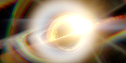
After quickly realizing that I could just ask Claude to accurately render a lens flare based on an optical prescription (a mathematical representation of a lens), I asked it to do so.

I had one major issue, though. Lens flare is based on how much light hits the sensor, and passes through the optical system. I couldn’t just take a PNG and give it lens flare. So, I went back, updated the renderer to output EXR files (essentially, multi-channel images with radiance data), and had Claude write up a physically-based lens flare simulator. I called it flaresim. Clever name, I know.

Over the course of a couple days, Claude and I worked to bring the tool to where it sits today. It can take any arbitrary EXR file, and any arbitrary optical prescription (I downloaded them from Photons to Photos) and output an EXR and TGA of the resultant image.

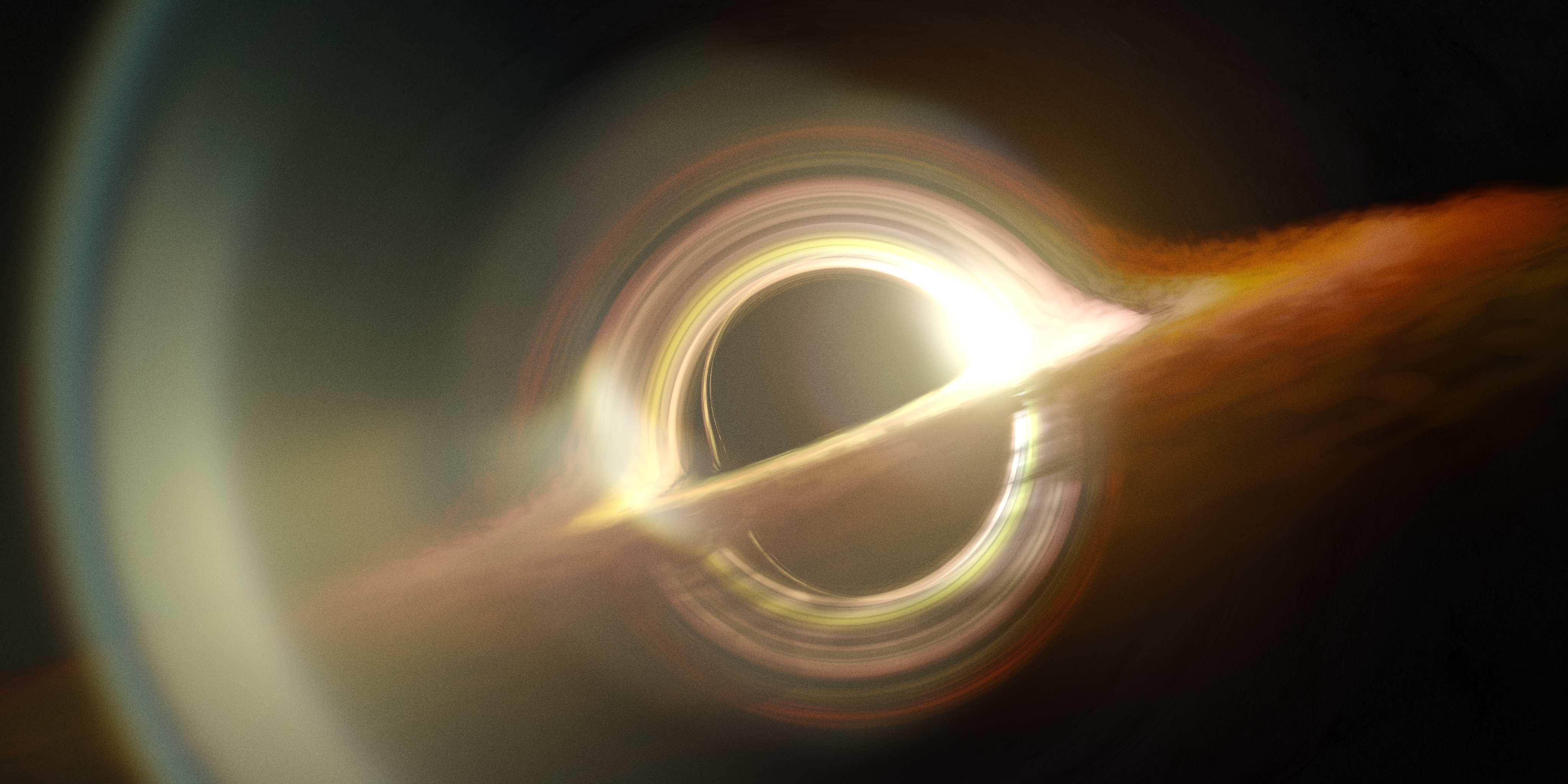
That is how I arrived at the below image.

The Finale #

This code was an awesome project, and gave me a lot of insight and experience with the tools and techniques I used to pull this off. The code is entirely open-source on my GitHub, and you can download it and create your own renders!